Step 23 of 40 - Financial Statement Formatting

Step 23 is intended to be a reinforcing step where you apply concepts covered previously in the assignment in the formatting of a Financial Statement.

Written description of the slides

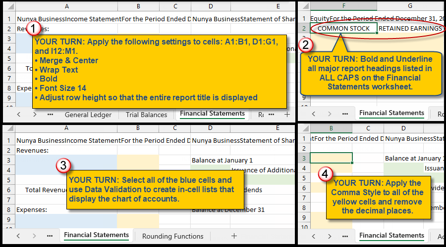
Step 1: Apply the formatting settings below to cells A1:B1, D1:G1, and I1:M1:

• Merge & Center
• Wrap Text
• Bold
• Font Size 14
• Adjust row height so that the entire report title is displayed.

Step 2: Bold and underline all major report headings listed in ALL CAPS on the Financial Statements worksheet.

Step 3: Select all of the blue cells and use Data Validation to create in-cell lists that display the chart of accounts.

Step 4: Apply the Comma Style to all of the yellow cells and remove the decimal places.

All of the concepts on Step 23 of 40 have been covered previously in the assignment:

• Merge & Center: #2 on Step 7 of 40                        
• Font Size 14: #4 on step 7 of 40
• Bold: #5 on Step 7 of 40
• Wrap Text: #7 on Step 7 of 40
• Adjust Row Height: #1 on Step 8 of 40
• Underline: #5 on Step 9 of 40
• Data Validation: Steps #1 through #12 on Step 21 of 40
• Comma Style: Steps #1 through #4 on step 10 of 40