Step 06 of 40: Freeze Panes Feature
This step illustrates how to use the Freeeze Panes feature in the View menu of Excel to keep certain rows (and/or columns) at the top (and/or left) of the worksheet grid so that headings and other wayfinding data don't scroll off of the screen.
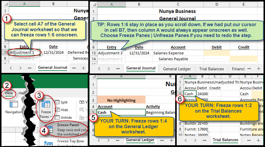
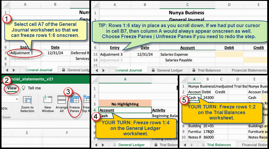
In Step 6, select cell A7 of the General Journal worksheet so that we can freeze rows 1:6 onscreen and choose View | Freeze Panes | Freeze Panes.
Freeze rows 1:4 on the General Ledger worksheet.
Freeze rows 1:2 on the Trial Balances worksheet.
TIP: Rows 1:6 stay in place as you scroll down. If we had put our cursor in cell B7, then column A would always appear onscreen as well. Choose Freeze Panes | Unfreeze Panes if you need to redo the step.
Steps labeled YOUR TURN are reinforcing steps that present opportunities to apply concepts covered earlier in the assignment.
We're here to help
If you're stuck or confused, send a copy of your workbook by way of one of these methods:
• Share: Click the Share command in the upper-right hand corner of the Excel screen, choose Share again, and then share the workbook with support@studentsexcel.com.
• Upload: You can upload a copy of your workbook at www.studentsexcel.com/student-upload.
• Email: You can email your workbook as an attachment to support@studentsexcel.com.
Be sure to listen to the audio portion of the video as you work through the assignment. The presenter elaborates further on what is being presented on screen and will offer tips.