Step 13 of 40: SUMIF Function
This step illustrates how to use the SUMIF Function to sum only the values for the entries in a given
Worksheet and Range that meet a certain Criteria (e.g., Accounts Payable).
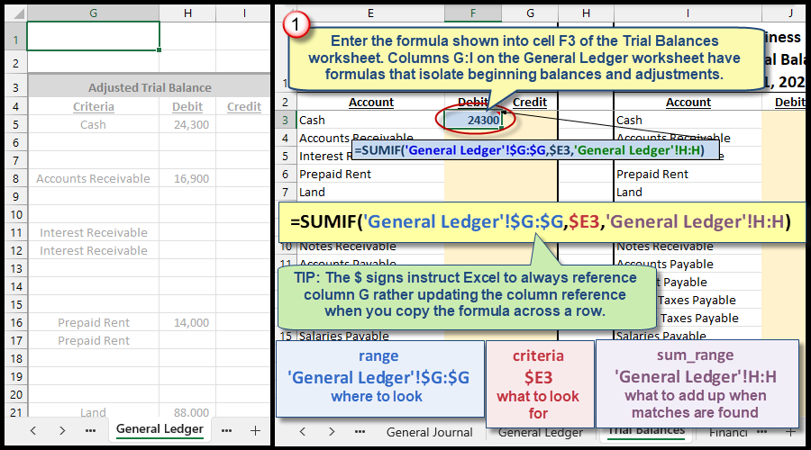
In Step 13, enter the formula =SUMIF('General Ledger'!$G:$G,$E3,'General Ledger'!H:H) into cell F3 of the Trial Balances worksheet. Columns G:I on the General Ledger worksheet have formulas that isolate beginning balances and adjustments.
- 'General Ledger'!$G:$G is the range that tells the formula where to look.
- $E3 is the criteria that tells the formula what to look for.
- 'General Ledger'!H:H is the sum_range that tells the formula what to add up when matches are found.
TIP: The $ signs instruct Excel to always reference column G rather updating the column reference when you copy the formula across a row.
Step-by-Step Instructions:
- Open the Trial Balances Worksheet:
Click on the Trial Balances tab at the bottom of the Excel workbook to activate it.
- Select Cell F3:
Click on cell F3 to make it the active cell where the formula will be entered.
- Start Entering the Formula:
Type =SUMIF( into cell F3. This begins the formula.
- Switch to the General Ledger Worksheet:
Now, click on the General Ledger worksheet tab at the bottom of the workbook to switch to that sheet.
- Select the First Range:
Highlight the G column by clicking the letter G at the top of the column. This represents the range you're summing based on the condition. You should now see ='General Ledger'!G:G appear in the formula.
- Press F4 (Windows) or Cmd+T (macOS) to lock the range, turning it into
='General Ledger'!$G:$G. This ensures the column reference is absolute (fixed).
- Return to the Trial Balances Worksheet:
Click on the Trial Balances tab again to switch back to this sheet.
- Now, click on cell E3 to refer to the criteria value.
You should now see E3 appear in the formula (this refers to the value you're comparing against).
- Press F4 (Windows) or Cmd+T (macOS) three times to lock the column, turning it into
='Trial Balance'!$E3or$E3. This creates a mixed cell reference, where the column is fixed, but the row number will change relative to where the formula is copied.
- Switch to the General Ledger Worksheet Again:
Click on the General Ledger tab again to switch back.
- Highlight the H column by clicking the letter H at the top of the column. This represents the values that will be summed if they meet the criteria.
- You should now see
'General Ledger'!H:Happear in the formula. Do not press F4 or Cmd-T this time because we want a relative cell reference such that the column letter will change relative to where the formula is copied.
- Complete the Formula by typing a closing parenthesis
)to complete theSUMIFformula.
- Press Enter or Return.
Press Enter or Return on your keyboard to confirm the formula.
The final formula should look like this:
=SUMIF('General Ledger'!$G:$G,$E3,'General Ledger'!H:H)
This formula will search column G of the General Ledger sheet for a value that matches E3 on the Trial Balances sheet, and if a match is found, it will sum the corresponding values from column H.

We're here to help
If you're stuck or confused, send a copy of your workbook by way of one of these methods:
• Share: Click the Share command in the upper-right hand corner of the Excel screen, choose Share again, and then share the workbook with support@studentsexcel.com.
• Upload: You can upload a copy of your workbook at www.studentsexcel.com/student-upload.
• Email: You can email your workbook as an attachment to support@studentsexcel.com.
Be sure to listen to the audio portion of the video as you work through the assignment. The presenter elaborates further on what is being presented on screen and will offer tips.
