Step 20 of 40: Sort Chart of Accounts

This step illustrates how to use the Custom Sort Function to sort a Chart of Accounts.

Written description of the slides

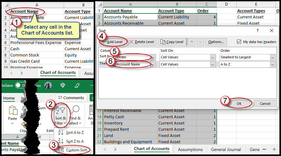
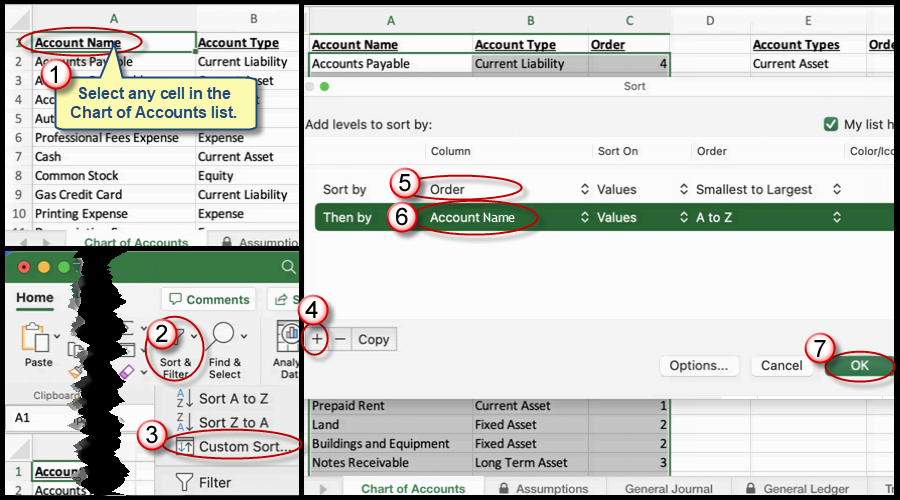
The Custom Sort Function sorts a worksheet according to specified criteria. In this case, you'll select any cell in the Chart of Accounts list and then choose Home | Sort & Filter | Custom Sort. In the Sort dialog box, choose Add Level, then select Order in the Sort By drop-down list, Account Name in the Then By drop-down list, and choose OK. Based upon these instructions, Excel will sort the Chart of Accounts according to this criteria.

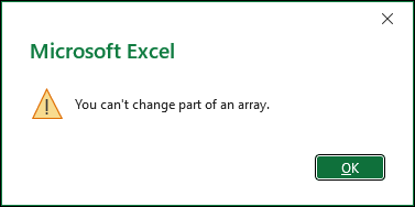
Troubleshooting the "You can't part of an array error"

Here's a breakdown of the formula as you likely wrote it:

=XLOOKUP(B2:B49, E$2:E$10, F$2:F$10)

• B2:B49 This is is a range of lookup values, which refers to the range where the formula will search for matching values. What is expected instead is to reference a single cell in this context, meaning B2.

  
  

• E$2:E$10: This is the lookup array. The function will search for values in this range to match with values in the B2:B49, or ideally just B2). The dollar signs before the row numbers (E$2:E$10) make the row references absolute, meaning they won't change when the formula is copied down.

  
  

• F$2:F$10: This is the return array. Once a match is found in the E$2:E$10 range, XLOOKUP will return the corresponding value from this range. The absolute references on the rows (F$2:F$10) mean the same return array will be used as the formula is copied down.

  
  

In summary:

The XLOOKUP function is matching each value in B2:B49 with values in E$2:E$10 and, if a match is found, returning the corresponding value from F$2:F$10.

The nuance that you've run into is that using a range, such as B2:B49, instead of just B2, creates a formula array within the spreadsheet. Formula-based arrays cannot be sorted. The easy fix is to change your formula to this:

=XLOOKUP(B29, E$2:E$10, F$2:F$10)

Once you've done so, click on cell C2 and double-click the Fill Handle, which will copy the formula down and then you'll be able to sort your results.