Step 38 of 40: Waterfall Chart Feature
This step illustrates how to use the Waterfall Chart Feature to display data.
Written description of the slides
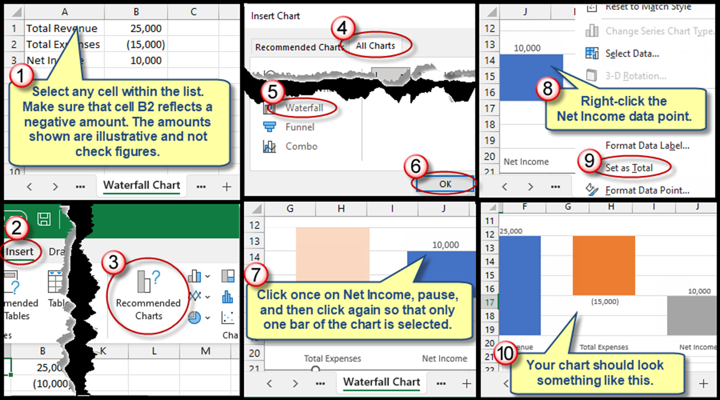
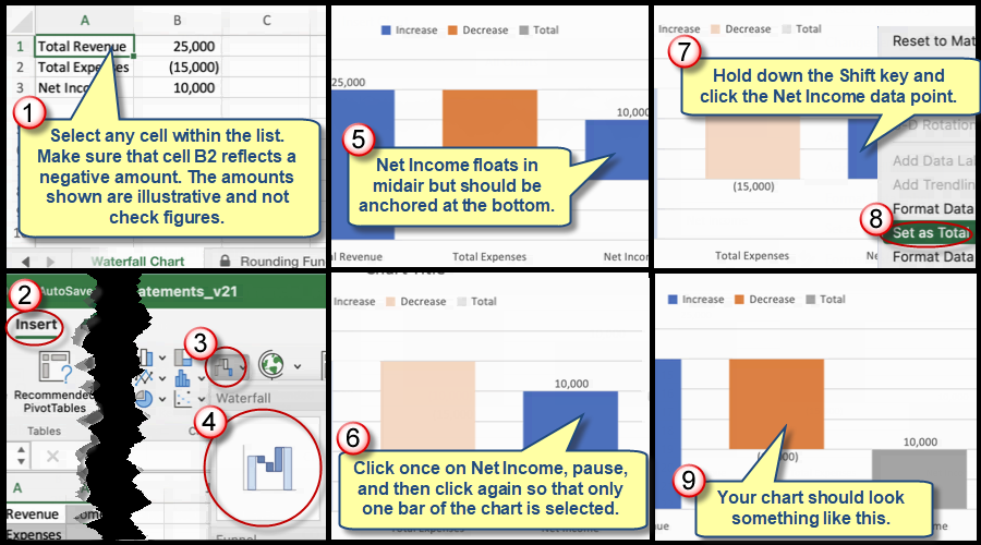
In Step 38, begin by selecting any cell within the list. Make sure that cell B2 reflects a negative amount. The amounts shown are illustrative and not check figures. Next, choose Home | Insert | Recommended Charts | All Charts | Waterfall and choose OK. Click once on Net Income, pause, and then click again so that only one bar of the chart is selected. Then, right-click the Net Income data point and choose Set as Total from the drop-down menu.
Your chart should look something like example in the last panel of the diagram below.
Steps labeled YOUR TURN are reinforcing steps that present opportunities to apply concepts covered earlier in the assignment.
We're here to help
If you're stuck or confused, send a copy of your workbook by way of one of these methods:
• Share: Click the Share command in the upper-right hand corner of the Excel screen, choose Share again, and then share the workbook with support@studentsexcel.com.
• Upload: You can upload a copy of your workbook at www.studentsexcel.com/student-upload.
• Email: You can email your workbook as an attachment to support@studentsexcel.com.
Be sure to listen to the audio portion of the video as you work through the assignment. The presenter elaborates further on what is being presented on screen and will offer tips.